Blog Feed

Game Theory: Overview

So today I am really inspired to write something about game theory in Mathematics, a very much thoroughly researched subject by mathematicians for a very long time, yet are so interesting for even beginners to the field. I would like to review some of the most basic definitions of game theories that I have learned as a student, followed by the review of common categories of games.

We start first with the primitive definition of game theory:

“Game theory is the study of mathematical models of strategic interaction among rational decision-makers.”

As you can see, this definition implemented that game theory is not just limited to the study of games and its mechanics, although this would later be an important part of crafting out the theories. The field focuses more heavily on strategies and logical reasoning, applying its results to model different types of behaviors and outcomes that can occur in real-life situations. This leads to an expansion in the definition of this term as the study of logical thinking among all individuals, but these expansions involve studies of other fields, which we will not focus on today.

Chess – a commonly research game

The question is: Why games?

If we consider games in the context of plays decided by skill, strength, or luck as in “football game”, this indeed can be frustrating. But if we consider the following definition of a game:

“A form of competitive activity played according to rules.”

then things are suddenly much more clear: any given conflict can actually be generalized into a game. The factors needed to form a game – players, rules, competitions – are already present in the conflict itself. Therefore, it is often in the best interests of mathematicians to research and model these situations in the form of games, as in those forms the numbers are much more easy to manage in the lack of context.

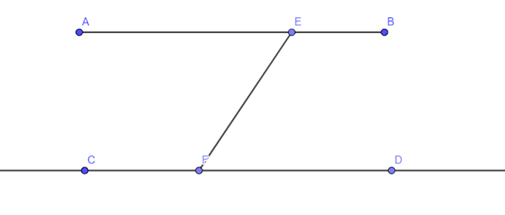
We will proceed to a classic example of a simplified real-life situation:

“Mum bought some candies which amount to a multiple of 5 and did not allow the babies to eat them. However, they broke the rules anyway, but each time, each baby can only take a number of candies anywhere from 1 to 4. Assuming that the baby competes for the last candy which is the best candy. Which baby has the strategy to win?”

However, when we rip off the context and generalize the numbers, we obtain the following version:

“A and B take turns to take candies. For each turn, a player would take a number of candies from 1 to n. Assuming that the number of candies is a multiple of (n+1) and the player taking the last candy wins. Which player has a guaranteed strategy to win?”

As you can see, the game is in a relatively generalized form (the number n might be defined as the maximum number of candies a baby can hold, etc.). With this version, we can now define several traits of the game:

  • The game is sequential: players are taking turns;
  • The game is non-cooperative: players may not form a mutual agreement;
  • The game is symmetric: changing players will not affect the overall result;
  • The game is evolutionary: players can change strategies according to recent moves;
  • The game has perfect information: players have exact records of all the events of the game.

which may specify ways of approaching the problem at hand. As of this example, the solution is quite simple:

The second player would have a guaranteed strategy to win by the following method: Whenever the first player picks a number of candies k between 1 and n, the second player would pick a number of candies equal to (n+1)-k. This method not only makes sure that the second player always has a response to the first player, but also means that the number of candies remaining after the second player’s turn will be a multiple of (n+1). As 0 is a multiple of (n+1), the second player would win.

Several portions of the solution can be attributed as a result of the traits. The strategy of the second player would not be possible without the perfect information trait, as it is dependent on knowing the very previous move of the first player. Moreover, the gameplay itself, and hence the strategy, is only feasible in the presence of the sequential and non-cooperative trait, because if the game had been either simultaneous or cooperative, the result would be very different.

Of course, games with traits different from the ones presented above are abundant. I would elaborate more on some of them, followed by examples in my later posts. For now, math on!

Mathematics vs. Physics: The Essentials

Mathematics and Physics, which is better?

Interestingly, I came upon these questions very often. Not only at school but also on the Internet as well. Like the other day when someone posted the very same thing, and boom, two opposite answers.

And surprisingly, both of them have their point. And the opposite of one’s strength is the other’s strength. And of course, none backs down.

As an observer, I find these discussions particularly interesting. It sure did highlight some of the differences between Maths and Physics, but I also believe that the peaceful coexistence of the two subjects is viable and vital through many interdisciplinary roles. Here are some takeaways

Math is more theoretical, while Physics is more practical:

To begin with, Mathematics is not observation-based. Its very nature is to derive conclusions, in this case, theorems, from a layer of other proven theorems, tracing back to a parent axiom which is universally agreed to be true. You just don’t really “observe” the theorems in real life, which leads to experiments holding minimal value in Mathematics, a feature unique to this particular subject. 

On the other hand, Physics, just like virtually any other science subject, is observation-based. In Physics, there is no axiom decided by humans, because nature does that job. This leads to a need to base theories on facts, and the ones which don’t are either rejected or remain hypotheses. Many times, a whole set of theories has to be rewritten because the foundation is proven wrong. And as more phenomena are observed, physics is always in a constant state of renewal to have fitting explanations to observations.

Physics can be relative, but Math has to be absolute:

Physics is a science that tries to explain nature, and nature, unfortunately, does not always operate by pattern. Therefore, no theory of Physics will ever be absolute truth; they are just not disproved yet. To adapt to this nature, physicians will happily accept theories that predict correctly a large number of observations, and will mostly still accept those theories if only a small number of opposing observations are found, only making small changes such as reducing the theories’ scope or adding exceptions. Logic is still needed but to a lesser degree.

Mathematics does not accept that kind of argument, as every one of its elements has to be logically defined. It deals with all things on a linear basis, and no theorem can be considered true while it is still undefined by preexisting theorems. On the other hand, if a theorem has been proven, that theorem will be an eternal truth – Mathematicians do not look back and revise it in any way. 

Mathematics is an abstract language; Physics is a realistic application

Of course, to sum up all characteristics, Mathematics is in itself a universal tool that can be applied to every other discipline. It proposes theorems without the need to depend on whether it would be useful – it just takes a complete analyses of ideas from their roots, which makes it powerful in terms of flexibility, but limited in terms of application. And while historically Mathematics had been devised from observations, modern Mathematics is increasingly turning to abstraction, and most of the researches nowadays cannot yet be utilized anywhere aside from pure Mathematics. This, however, will not deter them from possible applications in the future.

Adversely, Physics is specific in the very procedure of its operation from observation to theorizing to application. And as stated above, it tries to explain the nature, and none of its theory will, or even need to, go out of this bound. The standard practice of Physics, therefore, can be explained wholly by descriptions and patterns, but as this science explores deeper, this kind of approach proves inadequate compared to usage of Mathematics as a powerful tool. As it stands, applications of Mathematics in Physics are blooming, ranging from simple calculations to advanced probability and discrete Mathematics.

Conclusion:

As seen above, Mathematics and Physics can sometimes be polar-opposites, but are always supportive of the other – I have seen a lot of examples for this. Next time I’m talking more specifically on these applications, so stay tuned!

Imaginary and Complex Numbers

Imaginary numbers. It is not something that could be easily visualized – even its very name suggests so – but its presence in mathematics has been undeniable. Today, I will give an introduction to imaginary numbers, and some of its applications.

It is known for a fact that all real numbers, when squared up, yield positive numbers. That is why to have a result, a quadratic equation of the form:

ax^{2} + bx + c = 0

must satisfy, given that a is non-zero, the following criteria (non-negative discriminant):

b^{2} - 4ac \geq 0

Many equations don’t satisfy this condition, among those the seemingly very simple:

x^{2} + 1 = 0

In an effort to work around this drawback, a new concept must be introduced to find the roots of these equations – something that yields negative when squared up. Thus, the imaginary unit is born:

i^{2} = -1

So why “imaginary”? It’s simply because it’s not real. For every real number, you can always find a way to “visualize” it. A whole number is easy – for example an apple, two apples,… A fraction, or rational number, is harder, but still doable: for a fraction m/n, just split each apple into n equal parts and take m parts. Real number is hardest to imagine, but recalling a basic theorem gives us the way:

For every real number L, there exists a sequence of rational numbers that takes L as its limit.

Thus, we can imagine the apples being split indefinitely, and the result will approach the real number as it goes on. But you cannot imagine i apples – not even close. That’s because imaginary numbers are so different from the real ones that they, at least in a geometrical perspective, belongs to an entirely different dimension:

The complex number plane. The real number axis is horizontal, negative to the left, positive to the right. The imaginary number axis is vertical, negative downwards, positive upwards.

This concept allows mathematicians to discover a new type of number – complex numbers. They’re “complex” because they have two parts – the real part a and the imaginary part bi in the general representation:

a+bi

Geometrically, they have two be denoted in a plane (not an axis as for real numbers only), with two components giving it a two-dimensional nature. The most common one is to use the Descartes coordinates above, then a number of the form a+bi would be at the point (a, b).

Interestingly enough, the need for complex numbers did not arise due to quadratic equations. That’s because if one is only interested in real roots, then equations will real coefficients either have two roots or none. This is easily understandable: if one root of a quadratic equation is complex, the other must also be a complex root, since the sum of two roots is real according to the Vieta formula. This is aided by the fact that the general formula for the roots does not require complex numbers to be feasible. The case is different with cubic functions. Take the monic trinomial below that can be easily transformed to from the general cubic equation ax^{3} + bx^{2} + cx + d = 0 via the substitution x = t - \frac{b}{3a}:

t^3 + pt + q = 0

Now, the Cardano’s formula for general roots looks like this:

t_{k} = \alpha_{k} \sqrt[3]{-\frac{q}{2}+\sqrt{\frac{q^{2}}{4}+\frac{p^{3}}{27}}}+\alpha_{k}^{2}  \sqrt[3]{-\frac{q}{2}-\sqrt{\frac{q^{2}}{4}+\frac{p^{3}}{27}}}

with \alpha_{k}, k \in \{1, 2, 3\} being the three cube roots of 1, two of which is complex (the other is the trivial 1). So even if the equation has three real roots (for example, x^3-4x = 0 with roots 0, 2, -2), you still have to use complex numbers in order to find them using the generalized form. And that’s the true motive behind the first proper use of imaginary and complex numbers.

Luck, but… Statistically

Supposing one day you just walked out of your house and suddenly stepped on something and fell. When turning back to see who the “culprit” is, you suddenly faced a bill that someone has dropped.

You could totally say that you were “lucky”. More scientifically saying, you have just come across a series of random events whose results are positive to you. Actually, for each of us, perhaps encountering these series of events has become normal, and even some have encountered such repetitive series of events more than once.

So one question is asked: Are these series of events truly “accidental”? Is there any way to explain them? Moreover, how to optimize your luck? Let’s try to find the answer today!

Before we get to the analysis, the first two questions can easily be answered. These sequences are random, however, they do not fall from heaven. In fact, there is always a very small possibility set for each event. So when it comes to luck, actually we’re talking about this possibility, and when it comes to “optimizing luck”, we can understand it in one of two ways: either to improve it as much as possible or to predict this possibility most accurately to make the best decision.

Let’s take the example of a random event with different output cases. Each of these cases has a certain likelihood to occur, and this likelihood (or how we call it, “possibility”) is defined as the number of times we can get the desired result divided by the total number of tests, provided that the number of attempts has to be very large. Of course, the total possibility of different cases must be 1, or 100%.

So do we just need to refer to previous attempts to conclude the possibility of the incident, then decide whether or not to do it? Theoretically, this is completely true, but to apply this approach, we must first ensure all the conditions coincide. Assuming in the same test, if randomly circling all the sentences, you are then equally likely to have any mark from 0 to 10; however, if you study hard, the possibility you receive a bad mark will decrease significantly. Clearly, the difference in conditions, namely the amount of knowledge, has caused a change in the probability distribution of cases.

In fact, it is extremely difficult to find a sufficiently large sample of events with conditions that completely coincide so that an absolute true comparison can be made. Therefore, statisticians have decided to invent the standard deviation, which can be roughly interpreted as the amplitude of your “luck”. In any case, there is a 68% chance that it is within a radius of 1 standard deviation from the mean and 95% probability it is within a radius of 2 standard deviations. To know more about this, please kindly refer to the webpage on normal distribution in the references below.

So if you play a dart-throwing game at a fair 20 times, and statistics have shown that previous 20-turn players hit the target an average of 5 times with a standard deviation of 2 times, then you can rest assured that there is very low chance that you will not hit any of your shots – 95% of the time you will hit between 1 and 9 shots.

As you can see, even luck has its limits.

So in the end, how can we “optimize” our luck? According to the first understanding, we must improve the relevant factors, thereby improving the overall possibility. This in most cases is synonymous with reducing harmful factors. For example, in the coin-tossing game, you would like to reduce the width of the coin as much as possible to reduce the chance of it standing upright and resulting in neither heads nor tails, thereby improving your own chances of winning. It is worth mentioning that dirty plays also belong to this category of luck-improvement, as it improves your chances of winning by putting in beneficial factors.

By the second perspective, we have to increase the amount of data we have, thereby reducing the standard deviation and having a more accurate estimate of our “range of luck”. A relatively important concept regarding this is the confidence interval, which is basically a calculated interval with a high chance of containing the true probability. Let’s say, for instance, there is a game machine that we don’t know the winning probability, but if the 95% confidence interval is from 0.2 to 0.4, then there is 95% chance that this probability will fall from 0.2 to 0.4. In other words, don’t play, because you will be likely to lose more than you win. An important notice is that the confidence interval is inversely proportional to the square root of the sample size, therefore the more data we gather, the more accurate our prediction would be.

With these two ways, each of us can manage the risks in life better, or become “luckier”!

Music with Math? – Note Frequencies

Music and mathematics – if you happen to be involved in both of them, and there’s a high chance that anyone reading this has a background in both – then you sure have at least once heard of this pair. While neither originates from nor is a requirement for understanding the other, researching into the relationship between them has given quite some interesting results. However, today I will limit my discussion to a very basic overview of the frequencies of the notes you often hear.

  1. Why is frequency important?

As you all know, piano emits sounds when being played. Being a wave, sound has two properties: frequency and amplitude. The frequency affects the pitch of the sound, and the amplitude affects the volume. In the figure below we see the amplitude and wavelength of a typical sound wave, and the frequency value would equal the inversion of the wavelength value:

A sinusoidal sound wave, showing characteristics of wavelength (the... |  Download Scientific Diagram

There are many different notes, or pitches, and each of them comes with a different frequency. These frequencies, however, are strict, and it is important that the musical instrument follow it exactly in order to produce the sound needed. Therefore, knowing the frequency can greatly assist in tuning the instruments to its correct pitch.

  1. Frequency for Piano:

The modern piano people often see is based on the twelve-tone equal temperament system, containing the notes C, D♭, D, E♭, E, F, G♭, G, A♭, A, B♭, and B in that exact order, after which we will return back to C but one octave higher. This follows the octave rule, in which for every octave risen up, even though the note is the same, the frequency will be doubled, thus making it higher-pitched. Moreover, since the distance between the notes are geometrically (not arithmetically) equal, the frequency of each note will be a twelfth root of two higher than the previous note.

Fun Limit Problems – Not quite infinite!

Limits. This concept, with its explicit meaning “a point or level beyond which something does not or may not extend or pass”, is probably very familiar in real life. In Mathematics, limits are also very much the same despite its formal definitions having to use quite a number of Greek letters and signs, and such a concept has been inspired by or is applied in many interesting problems and phenomena. Today I will discuss two such problems I found interesting and relevant to the concept of limits: The Achilles and the Turtle paradox and the regular polygon area calculation. But first, let’s review the formal definitions.

  1. What is a limit?

The formal definition, or the {\displaystyle (\varepsilon ,\delta )} definition of limits, goes as follows:

Let {\displaystyle f} be a real-valued function defined on a subset {\displaystyle D} of the real numbers. Let {\displaystyle c} be a limit point of {\displaystyle D} and let {\displaystyle L} be a real number. We say that:

{\displaystyle \lim _{x\to c}f(x)=L}

if for every {\displaystyle \varepsilon >0} there exists a {\displaystyle \delta >0} such that, for all {\displaystyle x\in D}, if {\displaystyle 0<|x-c|<\delta }, then {\displaystyle |f(x)-L|<\varepsilon}.

Notice that we are dealing with limits here, so the function is not necessarily defined at {\displaystyle c}, and moreover {\displaystyle c} can be positive or negative infinite. To put it in an informal way, the definition implies that the limit is {\displaystyle L} if there is always a value attainable by the function that is near {\displaystyle L} enough, i.e. its difference to {\displaystyle L} is smaller than a specified value {\displaystyle \varepsilon >0} no matter how small {\displaystyle \varepsilon} can be.

  1. Achilles and the Turtle paradox:
One of very simple but confusing paradoxes involved in this book is the  paradox of Achilles and the Turtle. Achilles and the Tu… | Book projects,  Paradox, This book
Running as fast as he can, will Achilles overtake the turtle?

The Achilles and the Turtle paradox, one of those created by the ancient Greek Philosopher Zeno of Elea, was a perfect demonstration of how a seemingly infinite thing can never exceed a limited value. Let’s see the paradox after I have plugged in some numbers:

Achilles starts 10 meters behind the turtle. The turtle has the speed of 1 m/s, and Achilles has the speed of 10 m/s. Achilles will reach the starting point of the turtle in 1 second, in which time the turtle has crawled 1 meter. Achilles will have run that distance in the next 0.1 seconds, but the turtle has also crawled 0.1 meters in the meantime. Therefore, as the turtle is always in front of Achilles, he will never catch up to the turtle.

Of course we know that the statement is not true. Using physics, we can deduce that Achilles will catch up to the turtle in 

{10 / (10-1) = 1.111...} (seconds)

So why does the statement sound so true? Well, if you notice, the time intervals considered by the paradox are reduced by a factor of 10 each time (1 seconds to 0.1 seconds and so on). Calculating the limit to the sum of those intervals using the formula for geometric series {\dfrac{1}{1-q}}, we get the value 10/9. Therefore, the total time that the paradox considers will never reach 10/9 seconds, which is the time needed for Achilles to catch up to the turtle. 

This is often considered one of the earliest problems concerning limits (it comes sooner than the concept of limit for probably nearly 2 thousand years). The infinity property of the paradox, therefore, meant that this is not disproven for a very long time.

  1. Regular polygon’s area:
Demonstration of the area of circumscribed polygons. Notice how the blank area gets smaller.

As can be seen in the figure above, the area of the polygon comes closer to the area of the circle the more edges it gets. In other words, the limit of the area of a regular n-gon approaches a circle as n increases to infinity. This is because the formula of the area of a regular n-gon given its circumradius r is:

{\dfrac{r^{2}nsin(\dfrac{2\pi}{n})}{2}}

which equals to:

{\pi r^{2} \dfrac{n}{2\pi} sin(\dfrac{2\pi}{n})}


Taking the limit of the right side, using the standard limit {\lim_{x \to +\infty} \dfrac{1}{n} sin(n) = 1}, we would get the formula for the area of the circle. This is one of the most commonly known fun applications of limits.

Battleships!

Yo, what is this, a military force review? No of course, and while I can sit down and talk for hours about tanks and battleships (I do like them a lot) this is actually about the two-player board game Battleships, one of the games that (hopefully) you have played because you are missing out a lot of you don’t.

For anyone new to this game, you would be given a 10*10 board, on which you will have to place traditionally one 1*2 ship, two 1*3 ships, one 1*4 ship, and one 1*5 ship. Your placement will not be revealed to your opponent and vice versa, and the ultimate goal for both players would be to sink all enemy ships before all of your ships go down by correctly guessing the tile on which their ships are placed. Lots of variances are available to the format of the game, which truly makes playing it a rich experience. Today, I would like to look at the game strategies from a mathematical perspective, because believe it or not, your chance in this seemingly random game can be massively improved using probability calculation. 

Battleship (game) - Wikipedia
An example of a battleship game
  1. Offensive side – Guessing strategies:

The very basic first strategy is once you have managed a hit, immediately start playing around that square. Your second shot has a 25% chance of hitting (since you either play leftwards, rightwards, upwards, or downwards) and the third shot onwards until you sink the ship have a 50% chance of hitting each since you can continue the chain of blocks you have just formed. In every case, this is better than random potshots.

The second strategy theoretically reduces the number of moves you need to achieve a victory. If we color the battleship playground in a checkerboard pattern similar to the chessboard, a ship will always occupy at least one black square. Therefore, by attacking the black squares only, the player is assured to get hits in without resulting in random moves (you will be able to detect all enemy ships in below 50 moves a.k.a the number of black squares, which is just half of the board).

File:10x10 checkered board.svg - Wikipedia
Hit the black squares only!!

The third strategy is the evolutionary strategy. Remember that the way players choose squares to hit are not restricted by game rules, therefore players can adjust their strategies midway through the game, hence the term “evolutionary”. Suppose that you have sunk the 1*2 ship early in the game, and now all ships are 1*3 or longer. Therefore, you would like to avoid hitting 1*2 and 2*2 spaces since there is no longer a chance that a ship will appear inside it. Similarly, the dimensions of the spaces you would like to avoid will increase as you sink more ships, allowing you to focus your moves on other areas.

2. Game variations:

The variations to this game come in several types.

First is the board size, ship size, and ship number. This will heavily affect your chance of hitting, which is calculated by the number of target squares per the total number of squares. For the classic Battleships, the size of the board is 10*10 for a total of 100 squares, and the number of target squares is 17, so the hit chance is 17%. This brings about fast-paced gameplay, as the chance that you miss all 5 first shots are just 39%, way below average. Board variations can be n*n for any value of n, and the number of target squares can be changed by adding ships of the types above and even, in some cases, 2*3 aircraft carriers; but to design the most suitable experience, the hitting ratio will always have to be taken into account. Generally speaking, an initial hit ratio higher than 15% will lead to fast games, while an initial hit ratio lower than 10% will lead to long-winded battles. Moreover, due to the hit-around strategy, large ships are prone to be sunk very early, since they are easier to detect; therefore a game with a large number of small ships will always be slower than a game with a small number of large ships.

The second variation is in the number of shots per salvo, or the number of shots a player is allowed to fire in one turn. Choosing this variation will undoubtedly result in faster games, however, it is noteworthy that the more shots per salvo, the greater the advantage for the first player, since at any given time he will have fired more shots than the second player. For example, if the salvo has 5 shots, at the end of the first player’s turn he will be firing a total of 5 more shots than the second player, a gap that the second player can only breach after he ends his turn. Therefore, for maps with high hit ratios, the first player is prone to end the game faster due to the shots advantage. This makes salvo playing suitable only to low hit-ratio maps (below 10%) as with a long game the advantage will not be as noticeable.

The third variation and the one I like the most is the “ship-dependent” playstyle. In this mode, the number of shots per salvo equals the number of ships you have left. This game mode is fascinating as it directly rewards the sinking of ships with a massive advantage, and therefore demonstrates to the maximum the evolutionary strategy discussed above. Besides the normal approach of detection, a person can also choose to focus on big ships early on and sink them to give an advantage. For example, I always play with my friends a traditional setup of ships (17 target squares) but on a 15*15 board for a hit ratio of 7.55%, suitable for medium-to-long games even for salvo playstyle. I often ignore 3*3 squares from the get-go and instead just focuses on spaces that are 4 squares or longer, allowing me to pick up their 1*4 and 1*5 ships first and reduce their salvo size by 2. As you can see, this game mode focuses on obtaining a lead over the opponents as soon as possible and then builds upon that advantage, so using unorthodox strategies can be very beneficial.

I would like to end this writing with a fun math analysis of what would happen when the “ship-dependent” method above is applied to a high hit ratio map. Take the traditional map of 17% with 5 ships. Before the second player has the chance to do anything, the first player would have had a 61% chance of damaging at least one ship of the second player and a decent chance to sink at least one, especially if the hit-around method is applied. And there is a 1.2% chance that the first player sinks both the 1*2 and the 1*3 ship of the second player in his turn, reducing the second player’s salvo to 3 before the game even begins, which is a death sentence.

That’s why you don’t play salvo in high hit ratio maps!

Maximizing Efficiency – The Knapsack Problem

One of the most prominent aims, if not the most important, of Applied Mathematics lies in maximizing the efficiency of its subjects. Almost every industry and discipline in this world uses mathematical models to increase productivity as well as selecting the best targets for the given resources. This gives rise to a separate discipline of Applied Mathematics, namely Mathematical Optimization, which today we will look at along with one of its most important problems, the Knapsack Problem.

  1. What is Mathematical Optimization: 

A very formal definition would be:

“Mathematical optimization or mathematical programming is the selection of a best element (with regard to some criterion) from some set of available alternatives.”

From this definition, we can surely realize the very basic elements of what an optimization problem might look like. Of course there is the input, which are the ingredients or resources that you are willing to spend to achieve your goal. There are also given constraints which limits your options for your goal (for example, the constraint “bad weather” might prevent you from achieving your 10-kilometer run although the input – your strength – is enough provided that the weather is good). After passing your input through all the constraints, you will now possess a limited number or range of options, and the task for the mathematical model would be to select the best choice from those options.

Let’s look at an example below to see the interactions of input, constraints and output:

You are tasked to buy six kilograms of potatoes. There are two types you can buy: 2-kilogram bags costing $5 and 1-kilogram bags costing $3. Calculate the least amount of money to spend?

If all given data is just as above, we can easily deduce the least amount of money spent to be $15 by buying three 2-kilogram bags (the reason being that 2-kilogram bags cost less per kilogram at $2.5 compared to 1-kilogram bags at $3). However, if one more constraint is given:

The number of 2-kilogram bags must be smaller than 3.

then the answer changes to $16 (two 2-kilogram bags and two 1-kilogram bags). So constraints do greatly impact the results of optimization problems, and it is important that procedures adhere to them strictly to produce the best results.

Another question might be: Why is mathematical programming an alternative name to mathematical optimization? There are several reasons. First, mathematical optimization basically defines the operating procedures for the system to follow in order to achieve maximum results; so in some sense it basically “writes the program” for the system, resulting in the name. Secondly, mathematical optimization is easily one of the most computer-dependent branches of mathematics. Sure, we can calculate by hand the most simple of optimization problems, but for greater ones that can involve thousands of variables and inputs along with numerous constraints, it is ill-advised and sometimes even impossible to do so. With its impressive processing speed, computers are a much more viable way of approach, thus the name “mathematical programming”.

With that set, we can now proceed to one of the signature problems of the field.

  1. The Knapsack Problem:

or rather, how to fill the knapsack with the most value?

The Knapsack Problem and its variations are more often the most commonly found problems in Optimization, partly due to its rather non-specific requirements allowing for many different combinations of inputs and constraints to be used. The underlying idea is to fill the most valuable items, or any other objects with a value, into a fixed-size knapsack or any other given constraints. Among the variations, three generalizations are often recognized:

  • The 0-1 knapsack problem:

Given a set of \displaystyle {n} items numbered from 1 up to \displaystyle {n} , each with a weight \displaystyle {w_{i}} and a value \displaystyle {v_{i}} , along with a maximum weight capacity \displaystyle {W} ,

Maximize \displaystyle {\sum _{i=1}^{n}v_{i}x_{i}}

subject to \displaystyle {\sum _{i=1}^{n}w_{i}x_{i}\leq W} and \displaystyle {x_{i}\in \{0,1\}}

  • The bounded knapsack problem:

Basically a harder version of the 0-1 knapsack problem, the bounded knapsack problem replace the constraint of maximum one copy per item and instead replacing it with a predefined maximum number of copy for every item:

Maximize \displaystyle {\sum _{i=1}^{n}v_{i}x_{i}}

subject to \displaystyle {\sum _{i=1}^{n}w_{i}x_{i}\leq W} and \displaystyle {x_{i}\in \{0,1,...,c_{i}\}}

  • The unbounded knapsack problem:

The unbounded knapsack problem removes the maximum number of items altogether:

Maximize \displaystyle {\sum _{i=1}^{n}v_{i}x_{i}}

subject to \displaystyle {\sum _{i=1}^{n}w_{i}x_{i}\leq W}

Funnily enough, the example I gave above is a Knapsack problem. Did you spot it?

See you next week!

How to fall fastest? – The Brachistochrone Problem

Today I want to share with you one very fun application of optimization. Formally, it is called the Brachistochrone Problem, yet people can avoid remembering this long name by remembering the problem as “How to fall the fastest”. The problem was undoubtedly one of the most interesting at the time of introduction, and I thought it would be interesting to know the history behind one of probably the simplest applications of mathematics of all time.

  1. History of the problem:

For anyone who is interested, the name “Brachistochrone” is actually an Ancient Greek term meaning “shortest time”. The original statement of the problem, as posted by Johann Bernoulli in the first scientific journal of Europe Acta Eruditorum in June 1696, was:

“Given two points A and B in a vertical plane, what is the curve traced out by a point acted on only by gravity, which starts at A and reaches B in the shortest time.

Funnily enough, the problem was enclosed in a rather provocative challenge statement:

“Following the example set by Pascal, Fermat, etc., I hope to gain the gratitude of the whole scientific community by placing before the finest mathematicians of our time a problem which will test their methods and the strength of their intellect. If someone communicates to me the solution of the proposed problem, I shall publicly declare him worthy of praise.”

Of course, such an obvious natural phenomenon such as falling could not have been neglected all the way until 1696. Before that, Galileo Galilei, the same person who had proven that the falling speed for all objects is the same if not accounting for the air drag, had also considered the problem in 1638. However, due to calculus not having developed back then, Galileo’s solution of a circle arc passing through A and B was close, yet incorrect. 

Image 1: Illustrations of various considered curves (Source: maa.org)

In the end, 5 mathematicians responded to Johann’s problem statement: Isaac Newton, Jakob Bernoulli (Johann’s brother), Gottfried Leibniz, Ehrenfried Walther von Tschirnhaus and Guillaume de l’Hôpital. One of them in particular, Isaac Newton, showed his prowess by solving the problem in just a single day, and not only was he incorrect, his solution was also so unique that Johann recognized the author from the first sight. Regardless, the great number of responses to the problem did prove the extent of the development of calculus just 60 years after Galileo’s era, and paced the path for mathematics, especially optimization research, for years to come.

  1. Solution to the problem:

The answer for the problem is what would be later called a Brachistochrone curve, a version of the cycloid with the cusps pointing upward, starting at A – the beginning point – and ending at B –  the destination point. In turn, the cycloid is a curve equivalent to the path of a point on a circle when it is rolling on a surface: 

Image 2: How a cycloid is formed

There are various approaches to the problem, but almost all of them consider the velocity as the derivative of distance with regard to time. This particular consideration was undoubtedly one of the very first applications of calculus of variations (in this case, the distance) in order to find extremes (in this case, the smallest amount of time needed to reach the destination). It was Jacob Bernoulli’s solution and expansion of the problem that Leonhard Euler developed calculus of variations from, and later Joseph-Louis Lagrange, a famous French mathematician, would step in to create the modern infinitesimal calculus. The importance of the Brachistochrone problem, therefore, is to be emphasized and recognized throughout the history of Mathematics.

Graph Theory part 3 – Urban Planning

Graph theory plays an important role in mathematics, not only theoretically, but also realistically with its applications as well. One of those applications, and probably the most relatable one, is urban planning, where the most important thing is to find the most efficient pathing between two randomly given points. And if we consider the junctions as the vertices and the streets as the edges, we have ourselves a naturally-occurring giant graph that is the very city that we are living in. Last week, I wrote about the structural properties of graphs, including connectivity and several structure types (walks, trails, paths, cycles, and circuits). All of them are going to play in urban planning.

  1. Connectivity and circuitry – From the Seven Bridges of Konigsberg to modern days:

To us now, the visualization of streets as grids, facilitated by maps, is pretty much the standard;  but for the people back in the 1700s, when the roads system had not been extensively developed and so were the maps, it is debatable whether such a visualization was commonplace. Regardless, it was certain that research on graph theory was lackluster, and it was Leonhard Euler, the Swiss mathematician, who laid foundation for this field with his negative solution for the problem of the Seven Bridges of Konigsberg.

Above is a map of the seven bridges of Konigsberg at that time, along with the visualization of it as a graph with 4 vertices A, B, C, D. The challenge was simple: to complete a trip through all seven bridges without crossing any bridge twice, or, speaking with terminologies, to complete a trail of all edges of the graph. Many people have tried the challenge, but none managed to accomplish it – yet until Euler nobody was able to give a reason for their inability to do so. Before stepping into Euler’s solution, we consider this lemma:

A graph which exists a trail passing through all of its edges must either have:

  • Two odd-degree vertices, in which case the trail is open, or,
  • All even-degree vertices, in which case the trail is closed, or is a circuit.

Proving the lemma above is rather easy. In such a trail, every edge can be considered either an entering edge (in which the trail comes to the vertice after having passed through the edge) or an exiting edge (in which the trail comes to the vertice before entering the edge). So for every intermediate vertex (i.e. one that is not the beginning or the end of the trail), there must be an exiting edge for every entering edge, which makes the degree of the vertice even. In closed trails the ending and beginning of the trail is the same, so the degree of the beginning vertice is also even. In open trails, the beginning vertex has one more exiting edge than entering edge, and the ending vertex has one more entering edge than exiting edge, which makes their degree odd.

Coming back to the proof, Euler realized that all the vertices of Konigsberg had odd degrees (3 for B, C, D and 5 for A), which led him to the conclusion that the challenge was unsolvable, since there were 4 vertices of odd degrees in total.

What is the importance of this besides, well, laying the foundation for the entirety of graph theory, if it was not enough.

Take a look at city tours then.

Above is a map of a Ho Chi Minh city tour in Vietnam. Notice how there are no repeated streets except for that single entrance into the port on the right? Yep, there you go. Since tourist companies want to maximize the experience of their clients, it is in their absolute interest to constantly show new things on the way, and therefore not repeating the route is a must. Quite an interesting application of the problem hey?

  1. Minimizing the Distance:

There are multiple reasons why minimizing the distance is important. First, doing so has its economic benefits, including travelling time and fuel which can be converted into opportunity costs. Secondly, it also brings more comfort to the citizens, which would undoubtedly be irritated if forced to take a long runaround trip to get to their destination.

Regarding the best travelling route, it is common sense that the best route would always approach the destination either vertically or horizontally. For example, point B is on the top-right of point C, so a good route from B to D would always go up and right.

So why do we often see grid-like placement of the streets? Why not diagonal ones, which is always the best way of travelling?

The answer is: Using diagonal routes, while being an advantage to one, will be a disadvantage to another. In the example above, while CFEB is a good route to go from C to B, AEFB is a bad route to go from A to D, since the segment EF goes to the left instead of the right. In case of rectangular grids, everyone would be assured a good route.

Next week, I will probably write more on this fascinating topic – there is still so much to talk about. Math on!

Graph Theory part 2 – Structural Properties

Last week, I did an overview about graph theory, including two types of graphs: directed and undirected graphs. This time, I would like to dig further into some other forms that would define graphs more specifically than just the two overarching types above. Let’s see some of the structural properties of graphs for a more in-depth look.

  1. Connectivity:

The connectivity of a graph is decided by whether each pair of nodes in the graph are linked (i.e. there is a way to go between them, disregarding the direction of the edges in the cases or not). 

In the case of an undirected graph, if for every pair of nodes A and B there is a link between them, then it is connected.

In the case of a directed graph, things are a little bit more complicated, since you have to take into account the direction of the edges. There are, therefore, three levels of connectivity:

  • A strongly connected graph means that for every pair of nodes A and B, there is a way to go from A to B and a way to go from B to A. 
  • A weakly connected graph is a graph that would become connected if the directions of the edges are disregarded. In other words, there is at least one pair of nodes A and B that has no path between them, due to the arrows not following the intended way.
  • A unilaterally connected graph has at least a one-way link between every pair of nodes. So there exists at least a pair of nodes A and B that is not connected two-way, or else the graph would change to be strongly connected.

So, the levels of connectivity can be ranked as: 

Strongly connected > Unilaterally connected > Weakly connected

  1. Walk, Trail, Path, Cycle, and Circuit:

Why do those words sound kind of like synonyms?

Err, yes, but not in graph theory. They do have a similarity, however: All five of them are sequences of points and edges between those points. And that is pretty much it.

  • A walk is a sequence of vertices and edges. They can repeat, and they need not be closed. In the figure above, ABCEFCEC is a walk.
  • A trail is a walk that does not repeat edges. ABCE is a trail. ABCEA is a trail. ABCEC is not a trail. All trails are walks, but not the reverse.
  • A path is a trail but does not repeat vertices. So ABCE is a path, but ABCEA is not. All paths are trails and walks.
  • A cycle is a closed trail with no repeating vertices except for the beginning and the ending vertices. For example, ABCEA is a cycle.
  • A circuit is just a closed trail, so its vertices can repeat. For example, CFEDAEC is a circuit. All cycles are circuits.
  1. Complementary graphs:

The complementary graph of a graph G is the graph Gsuch that every connection missing in G is in GC but the two graphs have no common connection. Therefore, merging the two graphs together will create the complete graph. As demonstrated in the figure above, complementary graphs allow for two-way edges and self-loops (i.e. an edge with the same vertex as beginning and ending).

To construct the complementary graph of a graph, the method is to list down and then connect all the missing edges, and in the case of a directed graph, all the missing directions of existing edges as well.

Graph Theory

When we are talking about math, one of the easiest things to come to mind is its capacity for prediction, to help people plan. And most of the time, it is indeed the case, with prominent problems in this field being those involving finding the shortest distance, which is very useful for urban planning and economics. An advanced field of mathematics, despite not specifically designed for this, was one of its most significant contributors. Yes, I’m talking specifically about graph theory, a seemingly simple yet infinitely intricate, and interesting thing to study about. Let’s take a look!

  1. What is a graph?

The formal definition goes like this, at least for an undirected, simple graph:

graph is a pair G = (VE), where V is a set whose elements are called vertices, and E is a set of two-sets of vertices, whose elements are called edges.

To make a simple definition, imagine a set of dots, some of them connected. Notice how V is not a set of vertices, it is a set whose elements are called vertices. This means that the dots, or the vertices, are just the representations of the actual elements inside the V set. Similarly, the edges are just representations of the elements inside the set E. This clears up a lot about how graphs are usually used – the elements that needed describing will be the vertices, while the relationship between them will be the edges.

Take an example of a party, in which people take handshakes with each other. To track the handshakes, we would simplify the whole party into a single graph, in which:

  • V is the set of party attendants, each of whom is a vertex;
  • E is the set of handshakes, each of which is an edge.

In this graph-building method, the relationship between two elements of set V is defined as the handshake, a quantity that we would like to obtain – and thus comes the definition of set E.

2. Directed vs Undirected graphs:

In the first ‘handshake’ example, we saw how a graph can be constructed to symbolize the relationship between individuals or elements. However, it is worth noticing that a handshake does not give particular care to whether a person is a giver or receiver of the relationship. Many times, the relationship that needs to be accounted for has clear-cut givers and receivers, in which case the undirected graph would not be the best indicator.

This is where directed graphs are used. Direct graphs are almost identical in definition to undirected graphs, except that instead of edges, we have vectors to represent the set E. Therefore, the set now has defined givers and receivers as the beginning and ending points of vectors.

Consider documenting a graph for the example below:

A country has 12 cities, all of which are connected either directly or via some cities in between. Every city, however, can be the beginning of a maximum of 6 fly routes to other cities. Is such a configuration possible, and how can it be done?

We immediately see that one of the preconditions, being the beginning of a maximum of 6 fly routes to other cities, requires the use of a directed graph – without which we could not possibly know which city is the beginning of the flight route. With that in mind, we would construct a graph like this:

  • V is the set of cities, each of whom is a vertex;
  • E is the set of flying routes, each of which is a vector.

That is currently all I have to say. I hope I will catch you next week with more elaboration on this topic. Until then, math on!